Terraforma: Building Worlds with Perlin Noise and fBm

Published 2026/05/13 · rust · python · graphics

Procedural terrain is a common need in 3D graphical applications. Games such as Minecraft generate random, realistic landscapes to facilitate a unique, engaging experience with each world, and tech demos often showcase vast generated terrain.

These generated landscapes are built using fractional Brownian motion. fBm is a generalization of Brownian motion where increments are not necessarily independent, resulting in paths that remain rugged and random yet smoother than typical Brownian motion. The simulation of fractional Brownian motion has been the standard for terrain generation for decades due to the performance of the fBm approximation algorithm and the realistic results it achieves.

The most common fBm algorithm involves summating multiple samples of a noise function at various octaves. For each octave, the sample is taken with an exponentially increasing frequency and an exponentially decreasing amplitude. For landscapes, this is typically done in two dimensions, resulting in a heightmap that, when rendered as a model, resembles natural terrain. Terraforma takes a similar approach, performing fBm calculations with Perlin noise to generate convincing terrain.

Perlin noise

Perlin noise is the most common noise function for procedural terrain and graphics, and the noise function used in this project. First defined in An image synthesizer (1985) and later improved upon in Improving noise (2002), Perlin noise is a form of gradient noise designed to mimic the randomness found in the natural world. The algorithm can be described in these steps:

Assign a random gradient to each corner of the grid containing the point of interest.
Find the dot products between this gradient and the distance between the corner and the point.
Map each component point to a smoother line using some fade() function.
Using the faded point, interpolate in $N$ dimensions across the four dot products.

The Perlin noise implementation in Terraforma is object-based, so it must first be instantiated. This consists of creating a permutation array $P$ , where the integers 0-255 are shuffled. The array is then duplicated to avoid bounding errors. Accessing the permutations array allows for randomness that is consistent when accessing the same point.

pub fn new(seed: u64) -> Self {
    let mut rng = StdRng::seed_from_u64(seed);
    let mut permutations: Vec<usize> = (0..256).collect();
    permutations.shuffle(&mut rng);
    permutations.extend_from_slice(&permutations.clone()); // repeat in case of overflow
    Perlin { P: permutations }
}

The noise function starts by determining the given point $\vec{p}$ 's location within a box as well as the corners of the box. The boxes are each one square unit, so the new point is simply $\hat{p} = (x - ⌊ x ⌋, y - ⌊ y ⌋)$ .

After the points are calculated, the grad() function is called. The purpose of grad() is to find four dot products between the gradients of the corners and the point's distance from the corners. Based on the corner's coordinates, it chooses from one of four gradients: $(1, 1), (- 1, 1), (1, - 1), (- 1, - 1)$ . The gradient $\vec{g}$ is calculated as such, where $G$ is the array of possible gradients:

\vec{g} : = G [P [P [⌊ x ⌋] + ⌊ y ⌋] (\mod 4)]

Each corner then gets assigned the following dot product:

\vec{g} \cdot (\vec{p} - ⌊ \vec{p} ⌋)

fn grad(&self, trunc: [f64; 2], unit: [usize; 2]) -> (f64, f64, f64, f64) {
    let [x, y] = trunc;
    let [ux, uy] = unit;

    // pick gradient vectors for each corner
    let gtl = GRADIENTS[self.P[self.P[ux] + uy] & 3];
    let gtr = GRADIENTS[self.P[self.P[ux + 1] + uy] & 3];
    let gbl = GRADIENTS[self.P[self.P[ux] + uy + 1] & 3];
    let gbr = GRADIENTS[self.P[self.P[ux + 1] + uy + 1] & 3];

    // dot(gradient, distance)
    let dtl = dot2(gtl, [x, y]);
    let dtr = dot2(gtr, [x - 1.0, y]);
    let dbl = dot2(gbl, [x, y - 1.0]);
    let dbr = dot2(gbr, [x - 1.0, y - 1.0]);

    (dtl, dtr, dbl, dbr)
}

Then, $\vec{p}$ is mapped to a smoother function $fade (t) : = 6 t^{5} - 15 t^{4} + 10 t^{3}$ . The noise function then bilinearly interpolates over the dot products based on the faded point. Finally, the result is divided by $1 / \sqrt{2}$ to place the range between -1 and 1. The snoise() function retains this range, while the standard noise() function normalizes it to be between 0 and 1.

pub fn snoise(&self, x: f64, y: f64) -> f64 {
    // determine location within a box
    let trunc: [f64; 2] = [x - x.floor(), y - y.floor()];
    // determine in which box coordinates are located
    let unit: [usize; 2] = [(x as usize) & 255, (y as usize) & 255];
    // apply fade function to truncated coordinates
    let faded: [f64; 2] = trunc.map(|i| fade(i));

    let (dtl, dtr, dbl, dbr) = self.grad(trunc, unit);

    bilinear_interpolate(dtl, dtr, dbl, dbr, faded) / BOUND
}

Fractional Brownian motion

Let standard Brownian motion be defined as

B (t) = \int_{- \infty}^{t} W (s) d s

where $W (s)$ is a sample of white noise. Brownian motion has three main properties: a path that is continuous but not differentiable, independent increments, and stationary increments. This can be generalized into fractional Brownian motion, where increments are not necessarily independent. Its variance is described as

var (B_{H} (t_{2}) - B_{H} (t_{1})) \propto | t_{2} - t_{1} |^{2 H}

An additional component to fractional Brownian motion is the Hurst parameter $H$ , which describes the correlation of each increment in the following way, corresponding with the perceived roughness of the motion:

$H > 1 / 2$ : positive correlation
$H = 1 / 2$ : standard Brownian motion
$H < 1 / 2$ : negative correlation

While there are many methods for approximating fBm, the following method from Random Fractals in Image Synthesis (1991), inspired by Perlin's turbulence function, has become the go-to fBm approximation for the purposes of terrain generation (and many other forms of procedural graphics!):

B_{H} (x) = \sum_{k = 0}^{\infty} \frac{1}{Λ^{k H}} S (Λ^{k} x)

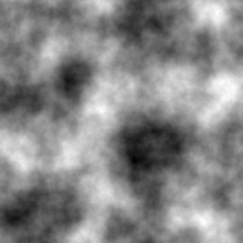
where $Λ$ is the lacunarity (a parameter that alters the frequency with each octave) and $S (x)$ is some sample, typically of a noise function. In most scenarios, the lacunarity is set to 2 and the Hurst exponent is set to 1, meaning that with each octave the image will become twice as detailed while each octave will have half the influence. This is the fBm approximation algorithm implemented in Terraforma, albeit with one tweak: the sum given by the fBm algorithm is divided by the sum of the amplitudes so that the values are guaranteed to be between 0 and 1. Here's my implementation:

pub fn fbm(
  x: f64, y: f64, period: f64, hurst: f64, lacunarity: f64, octaves: usize, p: &Perlin
) -> f64 {
    let mut total: f64 = 0.0;
    let mut amp_total: f64 = 0.0;
    let mut amp: f64 = 1.0;
    let mut freq: f64 = 1.0 / period;
    let gain: f64 = f64::powf(lacunarity, -hurst);
    for _ in 0..octaves {
        total += amp * p.noise(x * freq, y * freq);
        amp_total += amp;
        amp *= gain;
        freq *= lacunarity;
    }
    total /= amp_total; // guarantee within the range 0-1
    total
}

Here's the result:

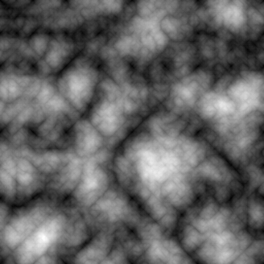
Some additional transformations are also available. There are contrast, exponent, and offset parameters to adjust the shape of the surface after the other calculations. In addition, the algorithm can be modified to use the absolute value of the signed noise to form valleys (see here for more):

for _ in 0..octaves {
    total += amp * p.snoise(x * freq, y * freq).abs();
    amp_total += amp;
    amp *= gain;
    freq *= lacunarity;
}
total /= amp_total; // guarantee within the range 0-1
total

which yields the following with Perlin noise:

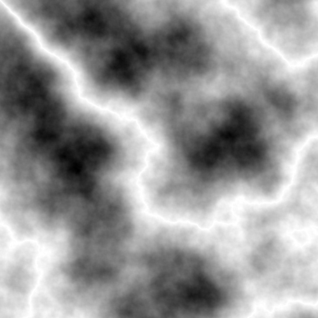
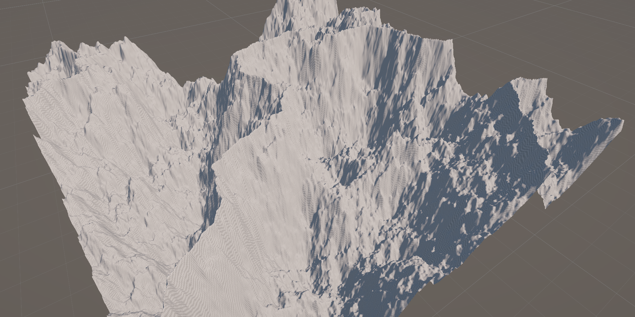
fBm heightmap with the valleys algorithm

Last but not least, taking the absolute value at the end and inverting the result forms sharp ridges that look electric:

for _ in 0..octaves {
    total += amp * p.snoise(x * freq, y * freq);
    amp_total += amp;
    amp *= gain;
    freq *= lacunarity;
}
total /= amp_total; // guarantee within the range 0-1
1.0 - total.abs()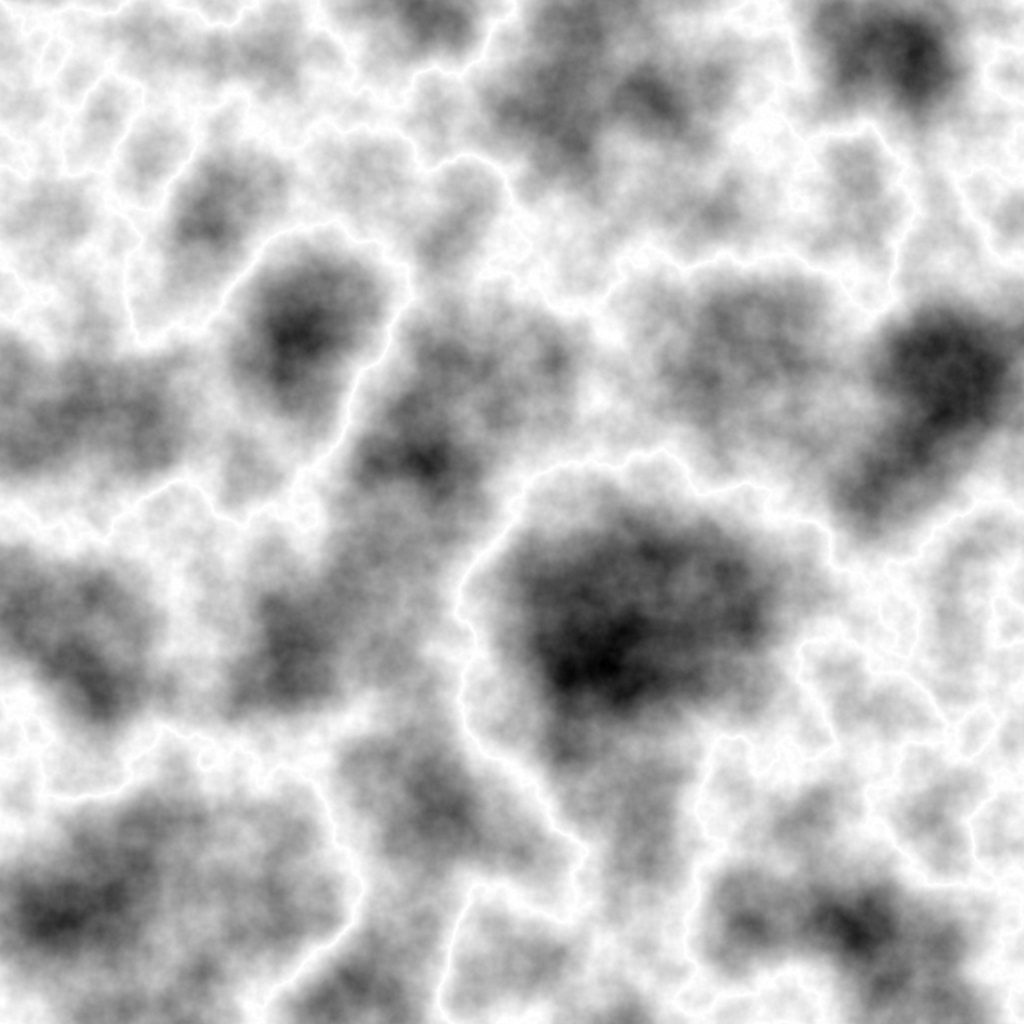

Importing into Unity

The nice thing about Terraforma is that it outputs a heightmap that can be used anywhere else, such as game engines. Because the program outputs an 8-bit PNG instead of a 16-bit RAW, if you want to use it in Unity you have to convert it to RAW (I used GIMP for this purpose). However, once you do that, it's really simple to just import and use:

The heightmap that was imported into Unity

A screenshot in the Unity Engine with the imported terrain

Future improvements

While I'm proud of what I've done so far with Terraforma, it still has a ways to go until I'm truly content with its state. For one, the current program is an ugly amalgamation of Python for the CLI and Rust for the calculations. This is an artifact of the original intent of it being written entirely in Python (It proved way too slow), but eventually I would replace the CLI with a TOML config file and build the heightmap using the image crate in Rust. If I really want to keep the other graphs generated by the Python script, it will be an entirely optional program run afterward.

Aside from the organization of the project, I also want to add more features. The main one I have in mind is extra noise functions, particularly value noise and simplex noise. Terraforma in its current state is already very versatile, but this will open even more possibilities.

That being said, this project was really fun to make and I can't wait to iterate on it even more!